Who this post is for

Here’s what I assume you to know:

• You’re familiar with R and the tidyverse.
• You know a little bit about fitting and evaluating linear regression models.

We will use the following R packages throughout this post:

library(MASS)
library(tidyverse)
library(tidymodels)

Generating some dummy data

Let’s get started by simulating some fake medical data for 100,000 patients. Assume we are interested in predicting their probability of death (=outcome). We use the patients’ sex (binary) and three continuous measurements — age, blood pressure , and cholesterol — to do so. In this fake data set, being female has a strong protective effect (odds ratio = exp(-2) = 0.14) and all other variables have a moderate effect (odds ratio per standard deviation = exp(0.3) = 1.35). Any influence by other, unmeasured factors is simulated by drawing from a Bernoulli distribution with a probability defined by sex, age, blood pressure, and cholesterol.

set.seed(42)

# Set number of rows and predictors
n <- 100000
p <- 3

# Simulate an additional binary predictor (e.g., sex)
sex <- rep(0:1, each = n %/% 2)

# Simulate multivariate normal predictors (e.g., age, blood pressure, 
# cholesterol)
mu <- rep(0, p)
Sigma <- 0.8 * diag(p) + 0.2 * matrix(1, p, p)
other_covars <- MASS::mvrnorm(n, mu, Sigma)
colnames(other_covars) <- c("age", "bp", "chol")

# Simulate binary outcome (e.g., death)
logistic <- function(x) 1 / (1 + exp(-x))
betas <- c(0.8, -2, 0.3, 0.3, 0.3)
lp <- cbind(1, sex, other_covars) %*% betas
death <- rbinom(n, 1, logistic(lp)) 

# Make into a data.frame and split into a training set (first half) and 
# a biased test set (rows in the second half X * beta > 0)
data <- as_tibble(other_covars)
data$sex <- factor(sex, 0:1, c("male", "female"))
data$pred_risk <- as.vector(logistic(lp))
data$death <- factor(death, 0:1, c("no", "yes"))
data$id <- 1:nrow(data)

Estimating predictive performance

Now that we have some data, we can evaluate how well our model is able to predict each patient’s risk of death. To make our lives as simple as possible, we assume that we were able to divine the true effects of each of our variables, i.e., we know that the data is generated via a logistic regression model with \(\beta = [0.8, -2, 0.3, 0.3, 0.3]\) and there is no uncertainty around those estimates. Under these assumptions, our model would be able to achieve the following AUC in the simulated data.

auc <- function(data) {
  yardstick::roc_auc(data, death, pred_risk, event_level = "second")
}

data %>% auc()

## # A tibble: 1 × 3
##   .metric .estimator .estimate
##   <chr>   <chr>          <dbl>
## 1 roc_auc binary         0.785

Notably, this is a summary measure that depends on the entire data set \(D\) and cannot be calculated for an individual patient alone. Per definition, it requires at least one patient with and without the outcome. This has important implications for interpreting the AUC. Let’s see what happens if we evaluate our (true) model in men and women separately.

men <- data %>% filter(sex == "male")
men %>% auc()

## # A tibble: 1 × 3
##   .metric .estimator .estimate
##   <chr>   <chr>          <dbl>
## 1 roc_auc binary         0.662

women <- data %>% filter(sex == "female")
women %>% auc()

## # A tibble: 1 × 3
##   .metric .estimator .estimate
##   <chr>   <chr>          <dbl>
## 1 roc_auc binary         0.665

In each subset, the AUC dropped from 0.78 to around 0.66. This perhaps isn’t too surprising, given that sex was a strong predictor of death. However, remember that the model coefficients and hence the predicted risk for each individual patient — i.e., how “good” that prediction is for that patient — remain unchanged. We merely changed the set of patients that we included in the evaluation. Although this might be obvious, I believe this is an important point to highlight.

Looking at the distribution of risks in the total data and by sex might provide some further intuition for this finding. Predicted risks for both those who did and did not die are clearly bimodal in the total population around the average risk for men and women (Figure 1). Even so, there is good separation between them. The majority of patients who died (red curve) had a predicted risk >50%. Vice versa, the majority of patients who remained alive (green curve) had a risk <50%. Looking at the risks of men and women separately, however, we can see that most men had a high and most women a low predicted risk (Figure 2). There is much less separation between the red and green curves, as any differences among for example the men is entirely due to moderate effects of our simulated continuous covariates.

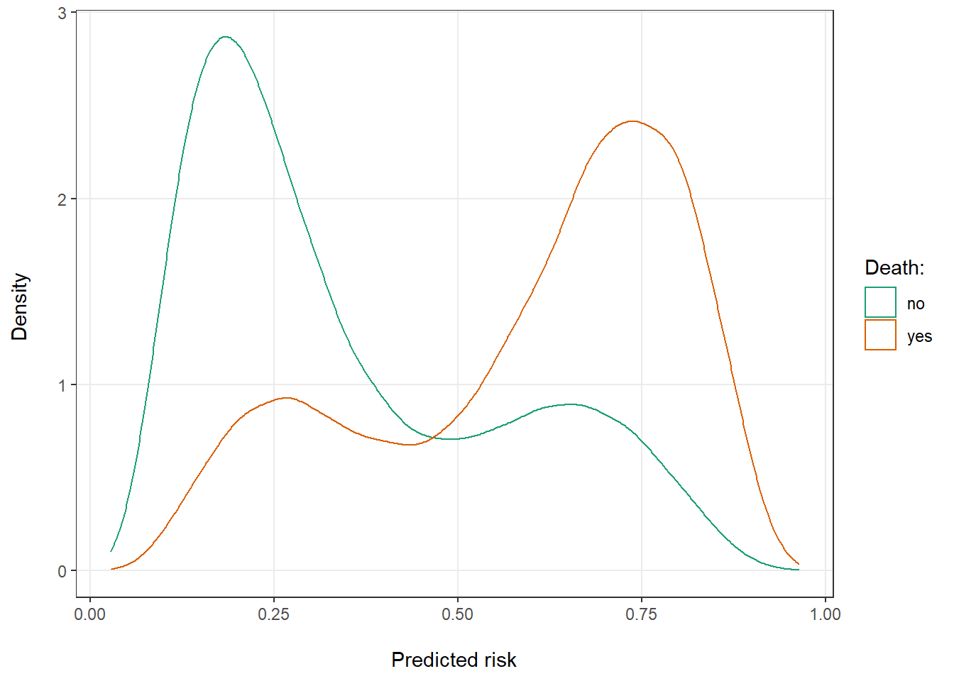
Figure 1: Distribution of predicted risk of death for patients that ultimately did and did not die.

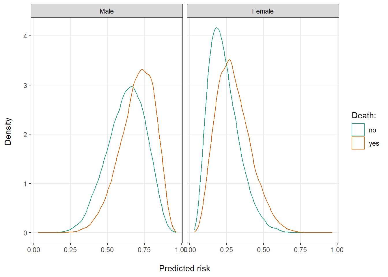
Figure 2: Distribution of predicted risk of death for by sex.

So far, we have looked at two extremes: the entire data set, in which sex was perfectly balanced, and two completely separated subsets with only men or only women. Let’s see what would happen if we gradually reduce the number of men in our evaluation population. We can see that estimated performance drops as we remove more and more men from the data set (Figure 3), particularly at the right side of the graph when there are only few men left and there is an increasing sex imbalance.

auc_biased <- function(data, p_men_remove) {
  n_men <- sum(data$sex == "male")
  n_exclude <- floor(n_men * p_men_remove)
  
  data %>% 
    slice(-(1:n_exclude)) %>% 
    auc()
}

p_men_remove <- seq(0, 1, by = 0.01)
auc_shift <- p_men_remove %>% 
  map_dfr(auc_biased, data = data) %>% 
  mutate(p_men_remove = p_men_remove)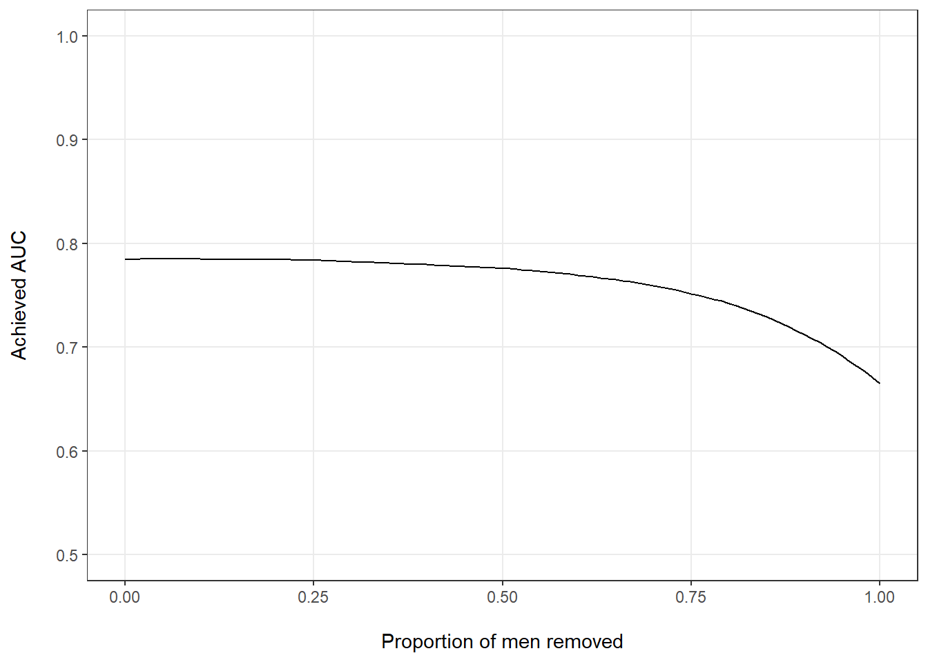

Figure 3: Estimated AUC by proportion of men removed from the full data set.

Difficulty to distinguish model misspecification

What we have seen so far is particularly problematic in the interpretation of external model validation, i.e., when we test a model that was developed in one set of patients (and potentially overfit to that population) in another patient population in order to estimate the model’s likely future performance. This is because in most real world cases, it isn’t quite as straightforward to quantify the difference between the development population and the evaluation cohort. Since we also usually don’t know the true model parameters (or even the true model class), it is difficult to disentangle the effects of population makeup from the effects of model misspecification. Let’s assume for example that — unlike earlier — we don’t know the exact model parameters and instead needed to estimate them from a prior development data set. As a result, we obtained \(\beta_{biased} = [0.8, -2, 0.3, 0.3, 0.3]\) which clearly differs from the true \(\beta\) used to generate the data. Now recalculate the AUC in a data set where there is some imbalance between men and women.

biased_betas <- c(0.4, -1, 0.3, -0.2, 0.5)
alt_risk <- logistic(cbind(1, sex, other_covars) %*% biased_betas) %>% 
  as.vector()

data %>% 
  mutate(pred_risk = alt_risk) %>% 
  auc_biased(0.5)

## # A tibble: 1 × 3
##   .metric .estimator .estimate
##   <chr>   <chr>          <dbl>
## 1 roc_auc binary         0.722

Again, the estimated model performance dropped. However, how much of the drop was due to our biased estimate \(\beta_{biased} \neq \beta\) and how much of it was due to the fact that our evaluation data set contained fewer men? This, in general, is not straightforward to answer.

Takeaway

If there is one takeaway from this post it is that external validations of predictive models mustn’t solely report on differences in AUC but also need to comment on the comparability of development and test sets used. Such a discussion is warranted irrespective of whether the performance remained the same, dropped, or even increased in the test set. Only by discussion — and ideally even quantifying — differences between the data sets can the reader fully assess the evidence for retained model performance and judge its likely value in the future.